Hasing table and Binary Tree

Hash Table is a data structure which stores data in an associative manner. In a hash table, data is stored in an array format, where each data value has its own unique index value. Access of data becomes very fast if we know the index of the desired data.

Thus, it becomes a data structure in which insertion and search operations are very fast irrespective of the size of the data. Hash Table uses an array as a storage medium and uses hash technique to generate an index where an element is to be inserted or is to be located from.

Hashing

Hashing is a technique to convert a range of key values into a range of indexes of an array. We're going to use modulo operator to get a range of key values. Consider an example of hash table of size 20, and the following items are to be stored. Item are in the (key,value) format.

• (1,20)
• (2,70)
• (42,80)
• (4,25)
• (12,44)
• (14,32)
• (17,11)
• (13,78)
• (37,98)

Sr.No.	Key	Hash	Array Index
1	1	1 % 20 = 1	1
2	2	2 % 20 = 2	2
3	42	42 % 20 = 2	2
4	4	4 % 20 = 4	4
5	12	12 % 20 = 12	12
6	14	14 % 20 = 14	14
7	17	17 % 20 = 17	17
8	13	13 % 20 = 13	13
9	37	37 % 20 = 17	17

Linear Probing

As we can see, it may happen that the hashing technique is used to create an already used index of the array. In such a case, we can search the next empty location in the array by looking into the next cell until we find an empty cell. This technique is called linear probing.

Sr.No.	Key	Hash	Array Index	After Linear Probing, Array Index
1	1	1 % 20 = 1	1	1
2	2	2 % 20 = 2	2	2
3	42	42 % 20 = 2	2	3
4	4	4 % 20 = 4	4	4
5	12	12 % 20 = 12	12	12
6	14	14 % 20 = 14	14	14
7	17	17 % 20 = 17	17	17
8	13	13 % 20 = 13	13	13
9	37	37 % 20 = 17	17	18

Basic Operations

Following are the basic primary operations of a hash table.

• Search − Searches an element in a hash table.
• Insert − inserts an element in a hash table.
• delete − Deletes an element from a hash table.

DataItem

Define a data item having some data and key, based on which the search is to be conducted in a hash table.

struct DataItem {
   int data;
   int key;
};

Hash Method

Define a hashing method to compute the hash code of the key of the data item.

int hashCode(int key){
   return key % SIZE;
}

Search Operation

Whenever an element is to be searched, compute the hash code of the key passed and locate the element using that hash code as index in the array. Use linear probing to get the element ahead if the element is not found at the computed hash code.

Example

struct DataItem *search(int key) {
   //get the hash
   int hashIndex = hashCode(key);
 
   //move in array until an empty
   while(hashArray[hashIndex] != NULL) {
 
      if(hashArray[hashIndex]->key == key)
         return hashArray[hashIndex];
   
      //go to next cell
      ++hashIndex;
  
      //wrap around the table
      hashIndex %= SIZE;
   }

   return NULL;        
}

Insert Operation

Whenever an element is to be inserted, compute the hash code of the key passed and locate the index using that hash code as an index in the array. Use linear probing for empty location, if an element is found at the computed hash code.

Example

void insert(int key,int data) {
   struct DataItem *item = (struct DataItem*) malloc(sizeof(struct DataItem));
   item->data = data;  
   item->key = key;     

   //get the hash 
   int hashIndex = hashCode(key);

   //move in array until an empty or deleted cell
   while(hashArray[hashIndex] != NULL && hashArray[hashIndex]->key != -1) {
      //go to next cell
      ++hashIndex;
  
      //wrap around the table
      hashIndex %= SIZE;
   }
 
   hashArray[hashIndex] = item;        
}

Delete Operation

Whenever an element is to be deleted, compute the hash code of the key passed and locate the index using that hash code as an index in the array. Use linear probing to get the element ahead if an element is not found at the computed hash code. When found, store a dummy item there to keep the performance of the hash table intact.

Example

struct DataItem* delete(struct DataItem* item) {
   int key = item->key;

   //get the hash 
   int hashIndex = hashCode(key);

   //move in array until an empty 
   while(hashArray[hashIndex] !=NULL) {
 
      if(hashArray[hashIndex]->key == key) {
         struct DataItem* temp = hashArray[hashIndex]; 
   
         //assign a dummy item at deleted position
         hashArray[hashIndex] = dummyItem; 
         return temp;
      } 
  
      //go to next cell
      ++hashIndex;
  
      //wrap around the table
      hashIndex %= SIZE;
   }  
 
   return NULL;        
}

To know about h

Binary Trees

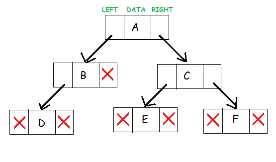
A binary tree is a hierarchical data structure in which each node has at most two children generally referred as left child and right child.

Each node contains three components:

1. Pointer to left subtree
2. Pointer to right subtree
3. Data element

The topmost node in the tree is called the root. An empty tree is represented by NULL pointer.

A representation of binary tree is shown:

---

Binary Tree: Common Terminologies

• Root: Topmost node in a tree.
• Parent: Every node (excluding a root) in a tree is connected by a directed edge from exactly one other node. This node is called a parent.
• Child: A node directly connected to another node when moving away from the root.
• Leaf/External node: Node with no children.
• Internal node: Node with atleast one children.
• Depth of a node: Number of edges from root to the node.
• Height of a node: Number of edges from the node to the deepest leaf. Height of the tree is the height of the root.

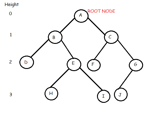
In the above binary tree we see that root node is A. The tree has 10 nodes with 5 internal nodes, i.e, A,B,C,E,G and 5 external nodes, i.e, D,F,H,I,J. The height of the tree is 3. B is the parent of D and E while D and E are children of B.

---

Advantages of Trees

Trees are so useful and frequently used, because they have some very serious advantages:

• Trees reflect structural relationships in the data.
• Trees are used to represent hierarchies.
• Trees provide an efficient insertion and searching.
• Trees are very flexible data, allowing to move subtrees around with minumum effort.

---

Types of Binary Trees (Based on Structure)

• Rooted binary tree: It has a root node and every node has atmost two children.
• Full binary tree: It is a tree in which every node in the tree has either 0 or 2 children.
  
  
  
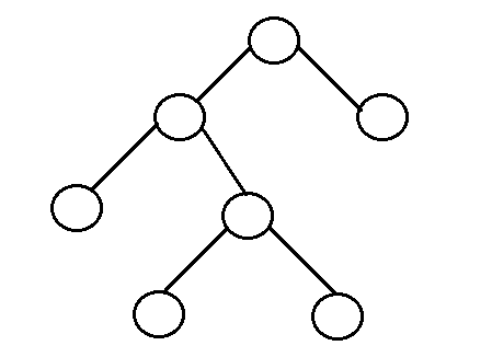
  • The number of nodes, n, in a full binary tree is atleast n = 2h – 1, and atmost n = 2h+1 – 1, where h is the height of the tree.
  • The number of leaf nodes l, in a full binary tree is number, L of internal nodes + 1, i.e, l = L+1.
• Perfect binary tree: It is a binary tree in which all interior nodes have two children and all leaves have the same depth or same level.
  
  
  
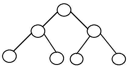
  • A perfect binary tree with l leaves has n = 2l-1 nodes.
  • In perfect full binary tree, l = 2h and n = 2h+1 - 1 where, n is number of nodes, h is height of tree and l is number of leaf nodes
• Complete binary tree: It is a binary tree in which every level, except possibly the last, is completely filled, and all nodes are as far left as possible.
  
  
  
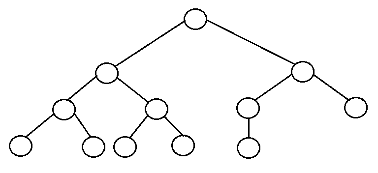
  • The number of internal nodes in a complete binary tree of n nodes is floor(n/2).
• Balanced binary tree: A binary tree is height balanced if it satisfies the following constraints:
  1. The left and right subtrees' heights differ by at most one, AND
  2. The left subtree is balanced, AND
  3. The right subtree is balanced
  An empty tree is height balanced.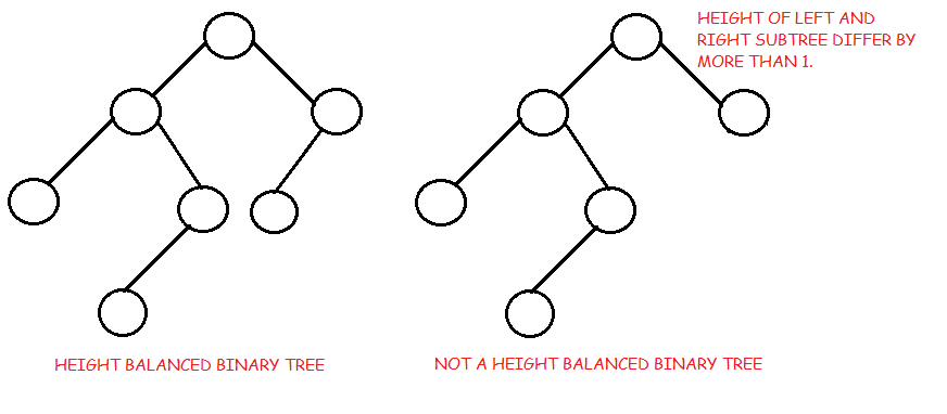
  
  
  
  • The height of a balanced binary tree is O(Log n) where n is number of nodes.
• Degenarate tree: It is a tree is where each parent node has only one child node. It behaves like a linked list.
  

---

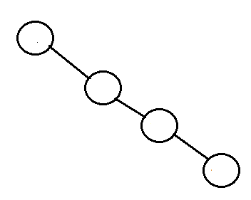
Binary Search Tree

A binary search tree is a useful data structure for fast addition and removal of data.
It is composed of nodes, which stores data and also links to upto two other child nodes. It is the relationship between the leaves linked to and the linking leaf, also known as the parent node, which makes the binary tree such an efficient data structure.
For a binary tree to be a binary search tree, the data of all the nodes in the left sub-tree of the root node should be less than the data of the root. The data of all the nodes in the right subtree of the root node should be greater than equal to the data of the root. As a result, the leaves on the farthest left of the tree have the lowest values, whereas the leaves on the right of the tree have the greatest values.
A representation of binary search tree looks like the following:



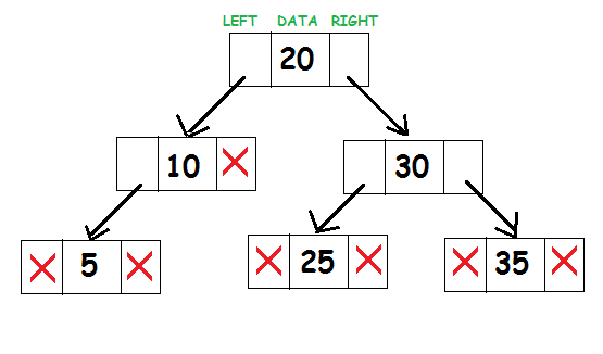
Consider the root node 20. All elements to the left of subtree(10, 5) are less than 20 and all elements to the right of subtree(25, 30, 35) are greater than 20.

---

Implementation of BST

First, define a struct as tree_node. It will store the data and pointers to left and right subtree.

struct tree_node
{
 int data;
 tree_node *left, *right;
};

The node itself is very similar to the node in a linked list. A basic knowledge of the code for a linked list will be very helpful in understanding the techniques of binary trees.
It is most logical to create a binary search tree class to encapsulate the workings of the tree into a single area, and also making it reusable. The class will contain functions to insert data into the tree, search if the data is present and methods for traversing the tree.

class BST
{
 tree_node *root;
 void insert(tree_node* , int );
 bool search(int , tree_node* );
 void inorder(tree_node* );
 void preorder(tree_node* );
 void postorder(tree_node* );

 public:
 BST()
 {
  root = NULL;
 }
 void insert(int );
 bool search(int key);
    void inorder();
    void preorder();
    void postorder();
};

It is necessary to initialize root to NULL for the later functions to be able to recognize that it does not exist.
All the public members of the class are designed to allow the user of the class to use the class without dealing with the underlying design. The functions which will be called recursively are the ones which are private, allowing them to travel down the tree.

---

Insertion in a BST

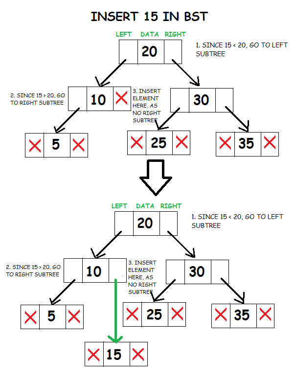
To insert data into a binary tree involves a function searching for an unused node in the proper position in the tree in which to insert the key value. The insert function is generally a recursive function that continues moving down the levels of a binary tree until there is an unused leaf in a position which follows the following rules of placing nodes.
• Compare data of the root node and element to be inserted.
• If the data of the root node is greater, and if a left subtree exists, then repeat step 1 with root = root of left subtree. Else,
• Insert element as left child of current root.
• If the data of the root node is greater, and if a right subtree exists, then repeat step 1 with root = root of right subtree.
• Else, insert element as right child of current root.




void BST :: insert(tree_node *node, int d)
{
 // element to be inserted is lesser than node’s data
 if(d < node->data)
 {
  // if left subtree is present
  if(node->left != NULL)
   insert(node->left, d);
  
  // create new node
  else
  {
   node->left = new tree_node;
   node->left->data = d;
   node->left->left = NULL;
   node->left->right = NULL;
  }
 }

 // element to be inserted is greater than node’s data
 else if(d >= node->data)
 {
  // if left subtree is present
  if(node->right != NULL)
   insert(node->right, d);
  
  // create new node
  else
  {
   node->right = new tree_node;
   node->right->data = d;
   node->right->left = NULL;
   node->right->right = NULL;
  }
 }
 
}

Since the root node is a private member, we also write a public member function which is available to non-members of the class. It calls the private recursive function to insert an element and also takes care of the case when root node is NULL.

void BST::insert(int d)
{
 if(root!=NULL)
                insert(root, d);
 else
    {
        root = new tree_node;
        root->data = d;
        root->left = NULL;
        root->right = NULL;
    }
}

---

Searching in a BST

The search function works in a similar fashion as insert. It will check if the key value of the current node is the value to be searched. If not, it should check to see if the value to be searched for is less than the value of the node, in which case it should be recursively called on the left child node, or if it is greater than the value of the node, it should be recursively called on the right child node.
• Compare data of the root node and the value to be searched.
• If the data of the root node is greater, and if a left subtree exists, then repeat step 1 with root = root of left subtree. Else,
• If the data of the root node is greater, and if a right subtree exists, then repeat step 1 with root = root of right subtree. Else,
• If the value to be searched is equal to the data of root node, return true.
• Else, return false.

bool BST::search(int d, tree_node *node)
{
 bool ans = false;

 // node is not present
   if(node == NULL)
   return false;
 
 // Node’s data is equal to value searched
    if(d == node->data)
       return true;
 
 // Node’s data is greater than value searched
    else if(d < node->data)
        ans = search(d, node->left);

 // Node’s data is lesser than value searched
    else
        ans = search(d, node->right);
  
    return ans;
}

Since the root node is a private member, we also write a public member function which is available to non-members of the class. It calls the private recursive function to search an element and also takes care of the case when root node is NULL.

bool BST::search(int d)
{
 if(root ==  NULL)
  return false;
 else 
  return  search(d, root);
}

---

Traversing in a BST

There are mainly three types of tree traversals:

1. Pre-order Traversal:

In this technique, we do the following :
• Process data of root node.
• First, traverse left subtree completely.
• Then, traverse right subtree.

void BST :: preorder(tree_node *node)
{
 if(node !=  NULL)
    {
  cout<<node->data<<endl;
        preorder(node->left);
        preorder(node->right);
    }
}




2. Post-order Traversal

In this traversal technique we do the following:
• First traverse left subtree completely.
• Then, traverse right subtree completely.
• Then, process data of node.

void BST :: postorder(tree_node *node)
{
 if(node !=  NULL)
    {
        postorder(node->left);
        postorder(node->right);
     cout<<node->data<<endl;
    }
}




3. In-order Traversal

In in-order traversal, we do the following:
• First process left subtree.
• Then, process current root node.
• Then, process right subtree.

void BST :: inorder(tree_node *node)
{
 if(node !=  NULL)
    {
        inorder(node->left);
     cout<<node->data<<endl;
        inorder(node->right);
    }
}

The in-order traversal of a binary search tree gives a sorted ordering of the data elements that are present in the binary search tree. This is an important property of a binary search tree.
Since the root node is a private member, we also write public member functions which is available to non-members of the class. It calls the private recursive function to traverse the tree and also takes care of the case when root node is NULL.

void BST :: preorder()
{
 if(root ==  NULL)
  cout<<"TREE IS  EMPTY\n";
 else
        preorder(root);
}

void BST :: postorder()
{
 if(root ==  NULL)
  cout<<"TREE IS  EMPTY\n";
 else
     postorder(root);
}

void BST :: inorder()
{
 if(root == NULL)
  cout<<"TREE IS EMPTY\n";
 else
  inorder(root);
}

---

Complexity Analysis




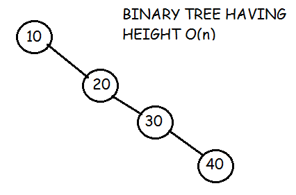
The time complexity of search and insert rely on the height of the tree. On average, binary search trees with n nodes have O(log n) height. However in the worst case the tree can have a height of O(n) when the unbalanced tree resembles a linked list. For example in this case :